感谢xxxxxin推荐的Graph-tool，看了画图效果之后被实力圈粉了。

1. Graph-tool是什么？

        Graph-tool is an efficient Python module for manipulation and statistical analysis of graphs (a.k.a. networks). Contrary to most other python modules with similar functionality, the core data structures and algorithms are implemented in C++, making extensive use of template metaprogramming, based heavily on the Boost Graph Library. This confers it a level of performance that is comparable (both in memory usage and computation time) to that of a pure C/C++ library.

        官网给出的几个画图效果。   2. 安装

        虽然是Python的一个库，但不能直接运行在windows系统上，尝试了brew install graph-tool 未果，转用了WSL Ubuntu 20.04, 添加镜像源的时候就是无法更新key，又不想用conda（每次安装感觉conda把我的python环境搞乱了，调试代码容易出错），最终选择用了docler 安装。以上背景陈述完毕，首先安装docker，具体操作可参考我的上一篇博客：Windows 10 安装 docker 记录。 安装好docker后，打开命令行（Win+R，输入cmd，然后Enter）安装graph-tool，命令如下：

docker pull tiagopeixoto/graph-tool

 PS：默认安装可能有点慢，解决方案参考：https://www.cnblogs.com/BillyYoung/p/11113914.html 添加阿里云或网易的镜像。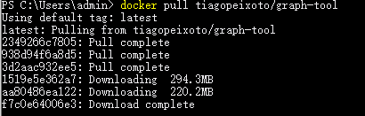

安装之后，运行：

docker run -it -u user -w /home/user tiagopeixoto/graph-tool ipython

运行之后是这样的：

>docker run -it -u user -w /home/user tiagopeixoto/graph-tool ipython
Python 3.8.3 (default, May 17 2020, 18:15:42) 
Type 'copyright', 'credits' or 'license' for more information       
IPython 7.15.0 -- An enhanced Interactive Python. Type '?' for help.

In [1]: 

这个用起来似乎不太方便，用个Jupyter notebook 吧，命令如下：

docker run -p 8888:8888 -p 6006:6006 -it -u user -w /home/user tiagopeixoto/graph-tool bash

然后再开启 notebook server：

jupyter notebook --ip 0.0.0.0

看控制台输出了访问地址，http://127.0.0.1:8888/?token=ea4de356a679fed6deb812ad79a3ed55015b604a6d99f794
就可以了。

3. 示例代码
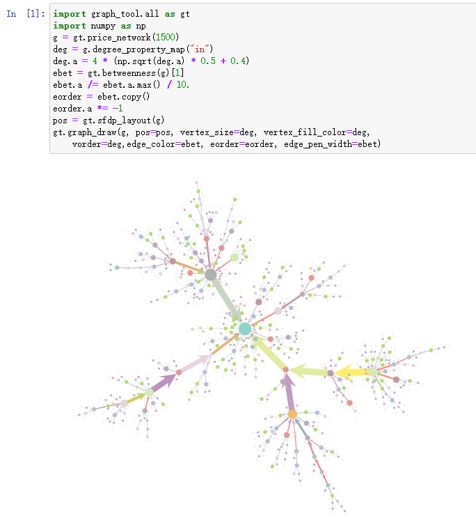
运行一段示例代码：  

import graph_tool.all as gt
import numpy as np
g = gt.price_network(1500)
deg = g.degree_property_map("in")
deg.a = 4 * (np.sqrt(deg.a) * 0.5 + 0.4)
ebet = gt.betweenness(g)[1]
ebet.a /= ebet.a.max() / 10.
eorder = ebet.copy()
eorder.a *= -1
pos = gt.sfdp_layout(g)
gt.graph_draw(g, pos=pos, vertex_size=deg, vertex_fill_color=deg,
    vorder=deg,edge_color=ebet, eorder=eorder, edge_pen_width=ebet,
    output="output.png")

再来看一下官网的示例代码：

#! /usr/bin/env python

# We will need some things from several places
from __future__ import division, absolute_import, print_function
import sys
if sys.version_info < (3,):
    range = xrange
import os
from pylab import *  # for plotting
from numpy.random import *  # for random sampling
seed(42)

# We need to import the graph_tool module itself
from graph_tool.all import *

# let's construct a Price network (the one that existed before Barabasi). It is
# a directed network, with preferential attachment. The algorithm below is
# very naive, and a bit slow, but quite simple.

# We start with an empty, directed graph
g = Graph()

# We want also to keep the age information for each vertex and edge. For that
# let's create some property maps
v_age = g.new_vertex_property("int")
e_age = g.new_edge_property("int")

# The final size of the network
N = 100000

# We have to start with one vertex
v = g.add_vertex()
v_age[v] = 0

# we will keep a list of the vertices. The number of times a vertex is in this
# list will give the probability of it being selected.
vlist = [v]

# let's now add the new edges and vertices
for i in range(1, N):
    # create our new vertex
    v = g.add_vertex()
    v_age[v] = i

    # we need to sample a new vertex to be the target, based on its in-degree +
    # 1. For that, we simply randomly sample it from vlist.
    i = randint(0, len(vlist))
    target = vlist[i]

    # add edge
    e = g.add_edge(v, target)
    e_age[e] = i

    # put v and target in the list
    vlist.append(target)
    vlist.append(v)

# now we have a graph!

# let's do a random walk on the graph and print the age of the vertices we find,
# just for fun.

v = g.vertex(randint(0, g.num_vertices()))
while True:
    print("vertex:", int(v), "in-degree:", v.in_degree(), "out-degree:",
          v.out_degree(), "age:", v_age[v])

    if v.out_degree() == 0:
        print("Nowhere else to go... We found the main hub!")
        break

    n_list = []
    for w in v.out_neighbors():
        n_list.append(w)
    v = n_list[randint(0, len(n_list))]

# let's save our graph for posterity. We want to save the age properties as
# well... To do this, they must become "internal" properties:

g.vertex_properties["age"] = v_age
g.edge_properties["age"] = e_age

# now we can save it
g.save("price.xml.gz")


# Let's plot its in-degree distribution
in_hist = vertex_hist(g, "in")

y = in_hist[0]
err = sqrt(in_hist[0])
err[err >= y] = y[err >= y] - 1e-2

figure(figsize=(6,4))
errorbar(in_hist[1][:-1], in_hist[0], fmt="o", yerr=err,
        label="in")
gca().set_yscale("log")
gca().set_xscale("log")
gca().set_ylim(1e-1, 1e5)
gca().set_xlim(0.8, 1e3)
subplots_adjust(left=0.2, bottom=0.2)
xlabel("$k_{in}$")
ylabel("$NP(k_{in})$")
tight_layout()
savefig("price-deg-dist.pdf")
savefig("price-deg-dist.svg")

运行结果： 再绘制一个多关系网络（graph-tool里的Layered network）

import graph_tool.all as gt
import numpy as np
import matplotlib

g = gt.collection.konect_data["ucidata-gama"]

# The edge types are stored in the edge property map "weights".

# Note the different meanings of the two 'layers' parameters below: The
# first enables the use of LayeredBlockState, and the second selects
# the 'edge layers' version (instead of 'edge covariates').

state = gt.minimize_nested_blockmodel_dl(g, layers=True,
                                         state_args=dict(ec=g.ep.weight, layers=True))

state.draw(edge_color=g.ep.weight, edge_gradient=[],
           ecmap=(matplotlib.cm.coolwarm_r, .6), edge_pen_width=5)

著名的美国大学生足球俱乐部网络（包含社团结构）：

import graph_tool.all as gt
import numpy as np

g = gt.collection.data["football"]
state = gt.PPBlockState(g)
# Now we run 1,000 sweeps of the MCMC with zero temperature.
state.multiflip_mcmc_sweep(beta=np.inf, niter=1000)
state.draw(pos=g.vp.pos)

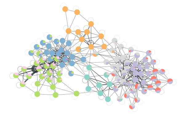
美国政治数据网络：

g = gt.collection.data["polbooks"]

state = gt.LatentMultigraphBlockState(g)

# We will first equilibrate the Markov chain
gt.mcmc_equilibrate(state, wait=100, mcmc_args=dict(niter=10))

# Now we collect the marginals for exactly 100,000 sweeps, at
# intervals of 10 sweeps:

u = None              # marginal posterior multigraph
bs = []               # partitions

def collect_marginals(s):
   global bs, u
   u = s.collect_marginal_multigraph(u)
   bstate = state.get_block_state()
   bs.append(bstate.levels[0].b.a.copy())

gt.mcmc_equilibrate(state, force_niter=10000, mcmc_args=dict(niter=10),
                    callback=collect_marginals)

# compute average multiplicities

ew = u.new_ep("double")
w = u.ep.w
wcount = u.ep.wcount
for e in u.edges():
    ew[e] = (wcount[e].a * w[e].a).sum() / wcount[e].a.sum()

bstate = state.get_block_state()
bstate = bstate.levels[0].copy(g=u)

# Disambiguate partitions and obtain marginals
pmode = gt.PartitionModeState(bs, converge=True)
pv = pmode.get_marginal(u)

bstate.draw(pos=u.own_property(g.vp.pos), vertex_shape="pie", vertex_pie_fractions=pv,
            edge_pen_width=gt.prop_to_size(ew, .1, 8, power=1), edge_gradient=None,
            output="polbooks-erased-poisson.svg")

海豚社交网络：

import graph_tool.all as gt
import numpy as np

# We will first simulate the dynamics with a given network
g = gt.collection.data["dolphins"]

# The algorithm accepts multiple independent time-series for the
# reconstruction. We will generate 100 SI cascades starting from a
# random node each time, and uniform infection probability 0.7.

ss = []
for i in range(100):
    si_state = gt.SIState(g, beta=.7)
    s = [si_state.get_state().copy()]
    for j in range(10):
        si_state.iterate_sync()
        s.append(si_state.get_state().copy())
    # Each time series should be represented as a single vector-valued
    # vertex property map with the states for each note at each time.
    s = gt.group_vector_property(s)
    ss.append(s)

# Prepare the initial state of the reconstruction as an empty graph
u = g.copy()
u.clear_edges()
ss = [u.own_property(s) for s in ss]   # time series properties need to be 'owned' by graph u

# Create reconstruction state
rstate = gt.EpidemicsBlockState(u, s=ss, beta=None, r=1e-6, global_beta=.1,
                                nested=False, aE=g.num_edges())

# Now we collect the marginals for exactly 1,000 sweeps, at
# intervals of 10 sweeps:

gm = None
bs = []
betas = []

def collect_marginals(s):
   global gm, bs
   gm = s.collect_marginal(gm)
   bs.append(s.bstate.b.a.copy())
   betas.append(s.params["global_beta"])

gt.mcmc_equilibrate(rstate, force_niter=1000, mcmc_args=dict(niter=10, xstep=0),
                    callback=collect_marginals)

print("Posterior similarity: ", gt.similarity(g, gm, g.new_ep("double", 1), gm.ep.eprob))
print("Inferred infection probability: %g ± %g" % (np.mean(betas), np.std(betas)))

# Disambiguate partitions and obtain marginals
pmode = gt.PartitionModeState(bs, converge=True)
pv = pmode.get_marginal(gm)

gt.graph_draw(gm, gm.own_property(g.vp.pos), vertex_shape="pie", vertex_color="black",
              vertex_pie_fractions=pv, vertex_pen_width=1,
              edge_pen_width=gt.prop_to_size(gm.ep.eprob, 0, 5))

4. 小结：

1. Graph_tool 是一个Python库，与大多数其他具有类似功能的python模块相反，核心数据结构和算法以C ++实现，大量使用了基于Boost Graph Library的模板元编程。 这赋予了它与纯C / C ++库相当的性能水平（在内存使用和计算时间上），因此效率高。
2. 绘图效果比较美观，自认为是目前绘图效果最好的工具包（超越了Gephi，d3.js，Python+Matplotlib，R绘图包，yEd，Pajek等一系列常见绘图工具）
3. 安装比较麻烦，Windows上可以使用conda或者docker或者WSL安装，但是docker相对简单一些
4. Graph_tool IO 首选格式是gt和基于文本的graphml，这两种格式都完全相同，但是gt格式更快，需要的存储量更少。完全支持 dot 和 gml 格式，但是由于它们不包含精确的类型信息，因此所有属性都将读取为字符串（对于gml，也将读取为双精度），并且必须手动将其转换为所需的类型。

参考资料：

1. https://graph-tool.skewed.de/
2. https://git.skewed.de/count0/graph-tool/-/wikis/installation-instructions#installing-using-docker
3. https://graph-tool.skewed.de/download
4. hub.docker.com查询images
5. 利用Graph-tool进行图的可视化处理